Background

Multiscale entropy (MSE) analysis [1,2] is a new method of measuring the complexity of finite length time series. This computational tool can be applied both to physical and physiologic data sets, and can be used with a variety of measures of entropy. We have developed and applied MSE for the analysis of physiologic time series, for which we prefer to estimate entropy using the sample entropy (SampEn) measure [3]. SampEn is a refinement of the approximate entropy family of statistics introduced by Pincus [4]. Both have been widely used for the analysis of physiologic data sets [5,6].

Traditional entropy measures quantify only the regularity (predictability) of time series on a single scale. There is no straightforward correspondence, however, between regularity and complexity. Neither completely predictable (e.g., periodic) signals, which have minimum entropy, nor completely unpredictable (e.g., uncorrelated random) signals, which have maximum entropy, are truly complex, since they can be described very compactly. There is no consensus definition of complexity. Intuitively, complexity is associated with ``meaningful structural richness'' [7] incorporating correlations over multiple spatio-temporal scales.

For example, we and others have observed that traditional single-scale entropy estimates tend to yield lower entropy in time series of physiologic data such as inter-beat (RR) interval series than in surrogate series formed by shuffling the original physiologic data. This happens because the shuffled data are more irregular and less predictable than the original series, which typically contain correlations at many time scales. The process of generating surrogate data destroys the correlations and degrades the information content of the original signal; if one supposes that greater entropy is characteristic of greater complexity, such results are profoundly misleading. The MSE method, in contrast, shows that the original time series are more complex than the surrogate ones, by revealing the dependence of entropy measures on scale [8,9,10,11,12].

The MSE method incorporates two procedures:

1. A ``coarse-graining'' process is applied to the time series. For a given time series, multiple coarse-grained time series are constructed by averaging the data points within non-overlapping windows of increasing length, $\tau$ (see Figure 1). Each element of the coarse-grained time series, $y^{(\tau)}_j$, is calculated according to the equation:
   

   $$y_j^{(\tau)}=1/\tau \sum_{i=(j-1)\tau+1}^{j\tau}x_i$$ (1)

   
   
   where $\tau$ represents the scale factor and $1\leq j \leq N/\tau$. The length of each coarse-grained time series is $N/\tau$. For scale 1, the coarse-grained time series is simply the original time series.

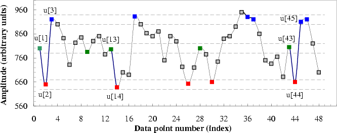
2. SampEn is calculated for each coarse-grained time series, and then plotted as a function of the scale factor. SampEn is a ``regularity statistic.'' It ``looks for patterns'' in a time series and quantifies its degree of predictability or regularity (see Figure 2).

Figure 1: Schematic illustration of the coarse-graining procedure for scale 2 and 3. Adapted from reference [8].

Figure 2: A simulated time series u[1], ..., u[n] is shown to illustrate the procedure for calculating sample entropy (SampEn) for the case in which the pattern length, m, is 2, and the similarity criterion, r, is 20. (r is a given positive real value that is typically chosen to be between 10% and 20% of the sample deviation of the time series.) Dotted horizontal lines around data points u[1], u[2] and u[3] represent u[1] $\pm$ r, u[2] $\pm$ r, and u[3] $\pm$ r, respectively. Two data values match each other, that is, they are indistinguishable, if the absolute difference between them is $\leq$ r. All green points represent data points that match the data point u[1]. Similarly, all red and blue points match the data points u[2] and u[3], respectively. Consider the 2-component green-red template sequence (u[1], u[2]) and the 3-component green-red-blue (u[1], u[2], u[3]) template sequence. For the segment shown, there are two green-red sequences, (u[13], u[14]) and (u[43], u[44]), that match the template sequence (u[1], u[2]) but only one green-red-blue sequence that matches the template sequence (u[1], u[2], u[3]). Therefore, in this case, the number of sequences matching the 2-component template sequences is two and the number of sequences matching the 3-component template sequence is 1. These calculations are repeated for the next 2-component and 3-component template sequence, which are, (u[2], u[3]) and (u[2], u[3], u[4]), respectively. The numbers of sequences that match each of the 2- and 3-component template sequences are again counted and added to the previous values. This procedure is then repeated for all other possible template sequences, (u[3], u[4], u[5]), ..., (u[N-2], u[N-1], u[N]), to determine the ratio between the total number of 2-component template matches and the total number of 3-component template matches. SampEn is the natural logarithm of this ratio and reflects the probability that sequences that match each other for the first two data points will also match for the next point.