Software Open Access
Logistic Regression-HSMM-based Heart Sound Segmentation
Published: July 29, 2019. Version: 1.0
New Software Package Added: HSS (April 10, 2016, midnight)
The Logistic Regression HSMM based Heart Sound Segmentation package contains MATLAB code used to segment phonocardiogram (PCG) recordings, and detect the four states of the heart cycle. This state of the art segmentation code by Springer is used in the sample entry of the 2016 PhysioNet/CinC Challenge.
When using this resource, please cite:
(show more options)
Springer, D. (2019). Logistic Regression-HSMM-based Heart Sound Segmentation (version 1.0). PhysioNet. https://doi.org/10.13026/vnt9-kf93.
Please include the standard citation for PhysioNet:
(show more options)
Goldberger, A., Amaral, L., Glass, L., Hausdorff, J., Ivanov, P. C., Mark, R., ... & Stanley, H. E. (2000). PhysioBank, PhysioToolkit, and PhysioNet: Components of a new research resource for complex physiologic signals. Circulation [Online]. 101 (23), pp. e215–e220.
Abstract
The identification of the exact positions of the first and second heart sounds within a phonocardiogram (PCG), or heart sound segmentation, is an essential step in the automatic analysis of heart sound recordings, allowing for the classification of pathological events. While threshold-based segmentation methods have shown modest success, probabilistic models, such as hidden Markov models, have recently been shown to surpass the capabilities of previous methods. Segmentation performance is further improved when apriori information about the expected duration of the states is incorporated into the model, such as in a hidden semi-Markov model (HSMM). This code provides Matlab algorithms to perform HSMM-based heart sound segmentation.
Background
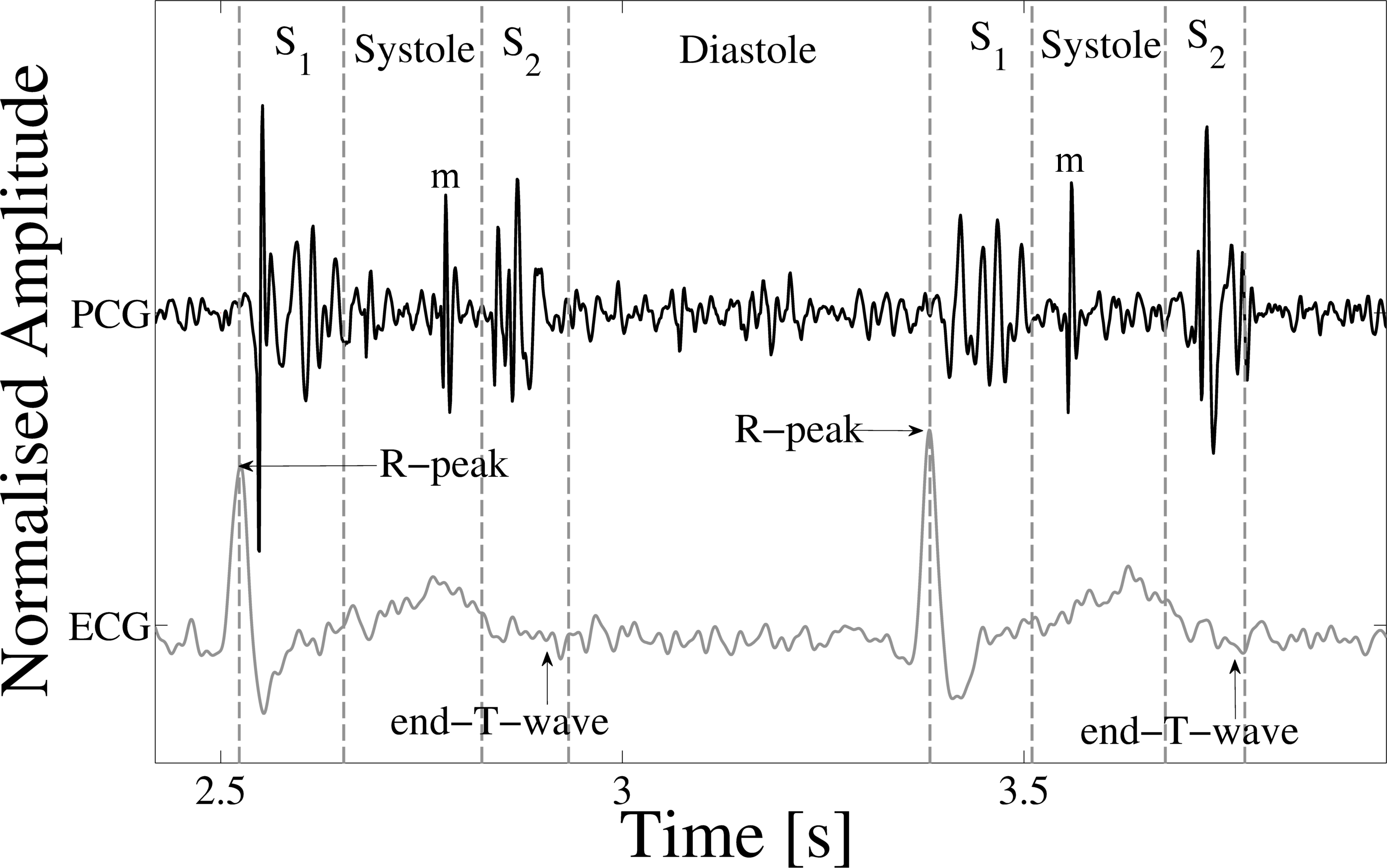
Heart sound segmentation refers to the detection of the exact positions of the first (S1) and second (S2) heart sounds in a heart sound recording or phonocardiogram (PCG). These sounds originate at the beginning of mechanical systole and diastole respectively [1], with S1 occurring immediately after the R-peak (ventricular depolarisation) of the electrocardiogram (ECG), while S2 occurs at approximately at the end-T-wave of the ECG (the end of ventricular depolarisation) [2] (See Figure 1).
Heart sound segmentation is an essential step in the automatic analysis of heart sound recordings, as it allows the analysis of the periods between these sounds for the presence of clicks and murmurs; sounds often indicative of pathology [3]. Segmentation becomes a difficult task when PCG recordings are corrupted by in-band noise. Common noise sources include endogenous or ambient speech, motion artefacts and physiological sounds such as intestinal and breathing sounds. Other physiological sounds of interest, such as murmurs, clicks, splitting of the heart sounds and additional S3 and S4 sounds, can also complicate the identification of the S1 and S2 sounds. For example, Figure 1 shows a PCG (alongside an ECG) with a loud mid-systolic click indicative of mitral valve prolapse, which could be confused for S1 or S2.
Figure 1 (in files below): Example of an ECG-labelled PCG, with the ECG, PCG and four states of the heart cycle (S1, systole, S2 and diastole) shown. A mid-systolic click can be seen in each of the heart cycles, labelled as "m". The R-peak and end-T-wave are labelled as references for defining the approximate positions of S1 and S2 respectively.
While threshold-based segmentation methods have shown modest success, probabilistic models, such as hidden Markov models (HMMs), have recently been shown to surpass the capabilities of previous methods. Segmentation performance is further improved when a priori information about the expected duration of the states is incorporated into the model, such as in a hidden semi-Markov model (HSMM) [4]. An excellent introduction to HMMs can be found in [5].
The code on this page extends the work of [4] by implementing such an HSMM for segmentation but extended with the use of logistic regression for emission probability estimation which was found to significantly improve segmentation accuracy. In addition, we implement a modified Viterbi algorithm for decoding the most-likely sequence of states. This modified Viterbi algorithm overcomes the limitation of the standard duration-dependant Viterbi algorithm where the start and end of detected states have to coincide with the start and end of the PCG recording. More details can be found in the paper referenced above.
Software Description
The code at the bottom of this page can be used to both train and execute the HSMM-based segmentation of PCGs. The step-by-step operations of the code are explained below.
Training the HSMM
The HSMM training is performed within the trainSpringerSegmentationAlgorithm.m file. Within this file, the basic steps are:
- Extract the features from the training set of recordings (
getSpringerPCGFeatures.m). These include the:- Homomorphic envelope
- Hilbert envelope
- Power spectral density envelope
- Discrete wavelet transform envelope
- Label the PCGs based on the supplied R-peak and end-T-wave locations (
labelPCGStates.m). - Train the three parameter matrices for the HSMM (
trainBandPiMatricesSpringer.m).
Running the trained HSMM
The three trained parameter matrices from above are used to segment a PCG in runSpringerSegmentationAlgorithm.m. The basic operations of the segmentation are:
-
Extract the features from a test set recording (
getSpringerPCGFeatures.m). -
Estimate the heart rate based on the autocorrelation (
getHeartRateSchmidt.m). - Use the extended duration-dependant Viterbi algorithm to derive the most likely sequence of states from the PCG (
lviterbiDecodePCG_Springer.m).- The duration distributions for the four states used in the Viterbi algorithm are computed in
get_duration_distributions.m.
- The duration distributions for the four states used in the Viterbi algorithm are computed in
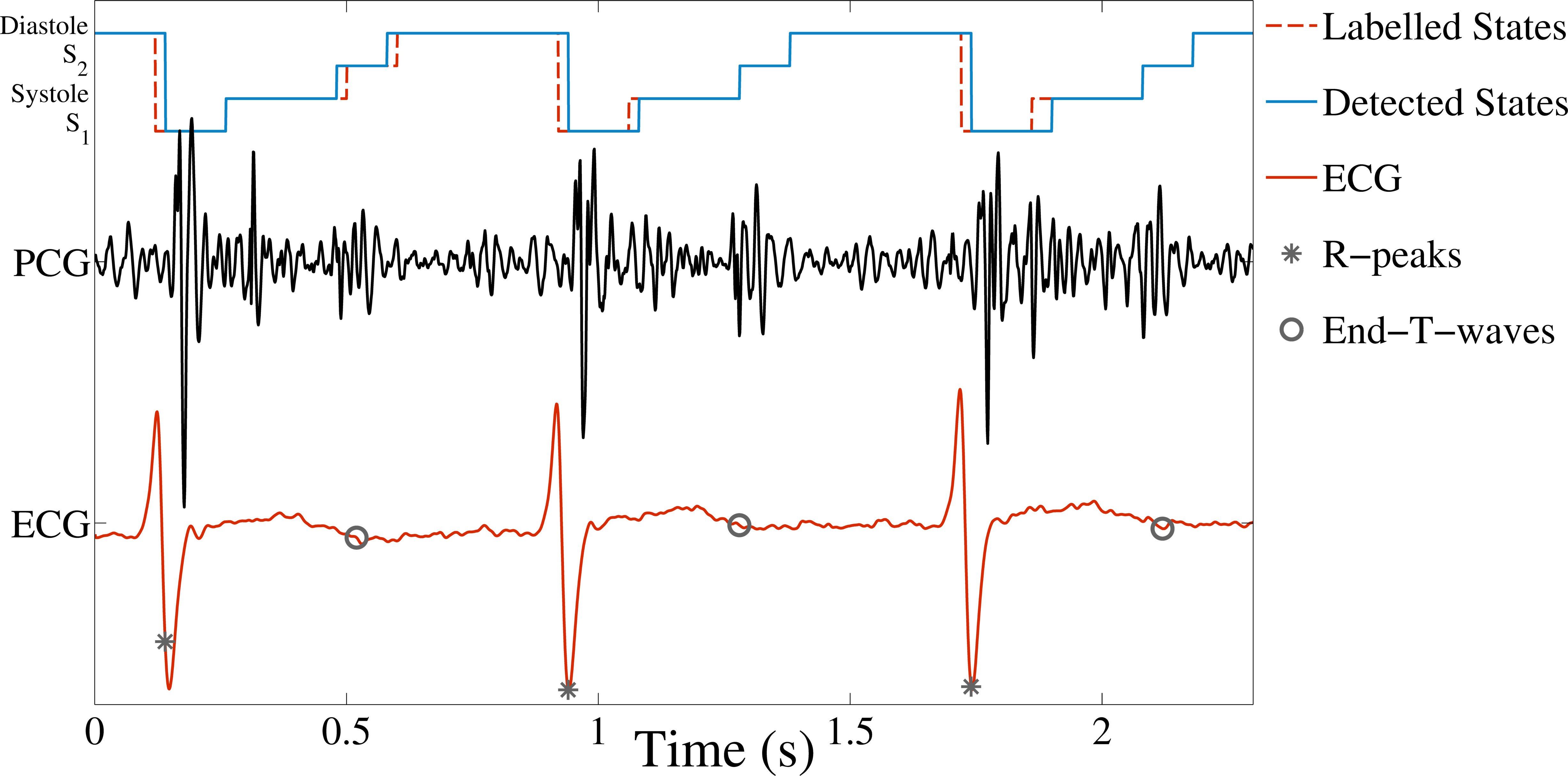
An example of the output of runSpringerSegmentationAlgorithm.m is shown in blue at the top of Figure 2.
Important options for the code are stored in default_Springer_HSMM_options.m. These include:
- The original sampling frequency of the PCG signals.
- The sampling frequency to which to downsample the segmentation features.
- Whether
.mexcode should be used for the Viterbi algorithm. - Whether wavelet features should be used (as this toolbox may be missing from your Matlab installation).
If you set springer_options.use_mex = true; in the options file, please be sure to run mex viterbi_Springer.c before running the code.
Figure 2 (in files below): Example of a segmented PCG using the code on this page. The four HSMM-detected states of the heart cycle (S1, systole, S2 and diastole) are shown at the top of the plot in blue - this is the output of the runSpringerSegmentationAlgorithm.m file. The red dotted line shows the labelled states, derived from the R-peak and end-T-wave positions in the labelPCGStates.m file. These labelled states are only used for training the algorithm. The ECG is shown in red at the bottom of the plot, with the positions of the R-peaks (*) and the end-T-waves (o) indicated. Only the PCG is used to derive the detected states in blue.
Installation and Requirements
An example of how the model is first trained on a small example set of data, and then used to segment a test recording is given in run_Example_Springer_Script.m. This should run out-of-the-box (provided you have set the default_Springer_HSMM_options.m correctly).
This code loads a few records from the example data. Alongside each recording are the R-peak and end-T-wave annotations which are used to label the locations of the heart sounds in the training set.
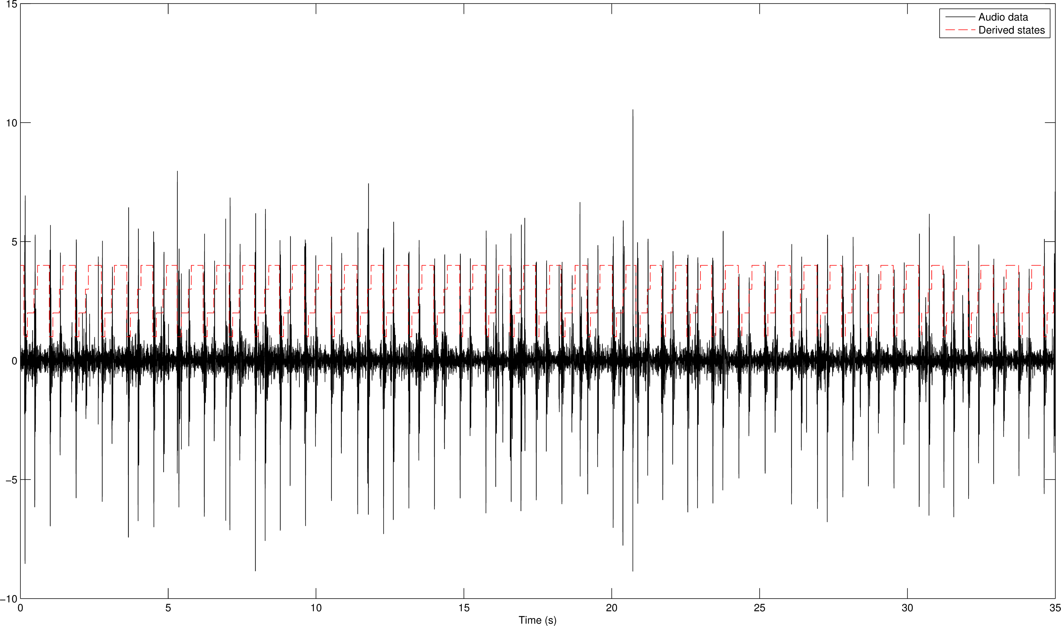
The HSMM is trained on five of the six example recordings, and applied to the sixth. Running this script should produce a plot similar to that shown in Figure 3.
Figure 3 (in files below): The output when running run_Example_Springer_Script.m. This shows the PCG signal in black, with the HSMM derived states shown in red.
The code in run_Example_Springer_Script.m will give you a clear example of how to apply these method to new datasets
Usage Notes
The example_data.mat file contains the full dataset from the paper mentioned at the top of this page. Included in this .mat file is a struct with the audio files, annotations, binary diagnosis (1 = presence of pathology) and the "patient number" for each record.
The example_data.example_audio_data is sampled at 1000 Hz, and contains recordings from various locations on the chest. While there are 135 patients, there are 792 recordings. This is due to multiple recordings per patient, as well as some recordings being split at positions of inconsistent annotations.
The example_data.example_annotations are the positions of the R-peak (first column of the cell array) and the end-T-wave positions (second column of the cell array), sampled at 50 Hz. As explained in the associated publication, these annotations are computed based on the agreement between five different automatic R-peak and end-T-wave detectors. They are not human-derived annotations.
The example_data.binary_diagnosis cell array shows which recordings were from subjects with no pathological heart damage as assessed by echocardiography (binary_diagnosis=0), and those with some sort of heart pathology (most commonly mitral valve prolapse - binary_diagnosis = 1).
The example_data.patient_number cell array indicates which subject each recording was captured from. Again, there are multiple recordings per patient due to multiple auscultation positions and splitting of recordings due to inconsistent annotations.
Conflicts of Interest
N/a
References
- Douglas, G., Nicol, E.F., and Robertson, C., Macleod’s Clinical Examination. Elsevier Health Sciences, 2009.
- Tilkian, A.G. and Conover, M.B., Understanding heart sounds and murmurs: with an introduction to lung sounds. Elsevier Health Sciences, 2001.
- Leatham, A. Auscultation of the heart and phonocardiography. Churchill Livingstone: 1975.
- Schmidt, S.E.; Holst-Hansen, C.; Graff, C.; Toft, E.; Struijk, J.J. Segmentation of heart sound recordings by a duration-dependent hidden markov model. Physiol Meas 2010, 31, 513-529.
- Rabiner, L., "A tutorial on hidden Markov models and selected applications in speech recognition," Proceedings of the IEEE, vol. 77, no. 2, pp. 257–286, Feb. 1989.
Access
Access Policy:
Anyone can access the files, as long as they conform to the terms of the specified license.
License (for files):
GNU General Public License version 3
Discovery
DOI (version 1.0):
https://doi.org/10.13026/vnt9-kf93
DOI (latest version):
https://doi.org/10.13026/9jqc-rv39
Programming Languages:
Corresponding Author
Files
Total uncompressed size: 147.9 MB.
Access the files
- Download the ZIP file (147.7 MB)
-
Download the files using your terminal:
wget -r -N -c -np https://physionet.org/files/hss/1.0/
-
Download the files using AWS command line tools:
aws s3 sync s3://physionet-open/hss/1.0/ DESTINATION